Calculating summary statistics¶

This page is a tutorial on calculating summary statistics from a libsequence.VariantMatrix. We also show how to interchange data between msprime [5] and pylibseq.

Simple overview of concepts¶

In [1]: import msprime

In [2]: import libsequence

In [3]: import numpy as np

# Get a TreeSequence from msprime
In [4]: ts = msprime.simulate(100, mutation_rate=250., recombination_rate=250., random_seed=42)

# TreeSequence -> VariantMatrix
In [5]: vm = libsequence.VariantMatrix.from_TreeSequence(ts)

# VariantMatrix -> AlleleCountMatrix
In [6]: ac = vm.count_alleles()

Certain summary statistics can be calculated simply from allele counts via libsequence.AlleleCountMatrix. Calculations invovling linkage disequilibrium will typically require the entire libsequence.VariantMatrix object.

The following examples rely on msprime [5] to generate input data, but the concepts hold more generally.

List of “classic”/standard summary statistics¶

Nucleotide diversity, or \(\pi\) [7]:

libsequence.thetapi(ac: libsequence._libsequence.AlleleCountMatrix) → float¶

Mean number of pairwise differences.

Parameters:	ac – A `libsequence.AlleleCountMatrix`

Note

Implemented as sum of site heterozygosity.

In [7]: print(libsequence.thetapi(ac))
980.3789898989783

Watterson’s estimator of \(\theta\), [10]:

libsequence.thetaw(ac: libsequence._libsequence.AlleleCountMatrix) → float¶

Watterson’s theta.

Parameters:	m – A `libsequence.AlleleCountMatrix`

Note

Calculated from the total number of mutations.

In [8]: print(libsequence.thetaw(ac))
982.5437651915445

Tajima’s \(D\), [8]:

libsequence.tajd(ac: libsequence._libsequence.AlleleCountMatrix) → float¶

Tajima’s D.

Parameters:	m – A `libsequence.AlleleCountMatrix`

In [9]: print(libsequence.tajd(ac))
-0.007527225314052745

Fay and Wu’s test statistic, \(\pi - \hat\theta_H\) [2] has two overloads. The first takes a single ancestral state as an argument. The latter takes a list of ancestral states (one per site in the variant matrix):

libsequence.faywuh(*args, **kwargs)¶

Overloaded function.

faywuh(ac: libsequence._libsequence.AlleleCountMatrix, ancestral_state: int) -> float
faywuh(ac: libsequence._libsequence.AlleleCountMatrix, ancestral_states: List[int]) -> float

In [10]: print(libsequence.faywuh(ac, 0))
-74.02989898988403

The \(H'\) statistic [11] should be preferred to the Fay and Wu test statistic:

libsequence.hprime(*args, **kwargs)¶

Overloaded function.

hprime(ac: libsequence._libsequence.AlleleCountMatrix, ancestral_state: int) -> float
hprime(ac: libsequence._libsequence.AlleleCountMatrix, ancestral_state: List[int]) -> float

In [11]: print(libsequence.hprime(ac, 0))
-0.12962968409194914

Summaries of haplotype variation [1]:

libsequence.number_of_haplotypes(arg0: libsequence._libsequence.VariantMatrix) → int¶

libsequence.haplotype_diversity(arg0: libsequence._libsequence.VariantMatrix) → float¶

In [12]: print(libsequence.number_of_haplotypes(vm))
99

In [13]: print(libsequence.haplotype_diversity(vm))
0.9997979797979798

The \(nS_L\) and \(iHS\) “haplotype homozygosity” statistics defined in [3]:

libsequence.nsl(m: libsequence._libsequence.VariantMatrix, refstate: int) → libsequence._libsequence.VecnSLResults¶

This function returns a list of instances of the following:

class libsequence.nSLresults¶

Holds nSL, iHS, and non-reference count at core SNP

core_count¶: Core mutation count in sample

ihs¶: iHS

nsl¶: nSL

Values of nan imply that haplotype homozygosity for a particular core variant was not broken within the matrix. This is the same procedure used in [3]. The return value order corresponds to the row order of the input data:

In [14]: nsl = libsequence.nsl(vm, 0)

In [15]: for i in nsl[:4]:
   ....:    print(i.core_count, i.ihs, i.nsl)
   ....: 
1 nan nan
8 nan nan
3 nan nan
7 -0.09735588583687971 -0.5544227795580867

The following variant only allows haplotype homozygosity to be broken up by mutations where the non-reference count is \(\leq x\):

libsequence.nslx(m: libsequence._libsequence.VariantMatrix, refstate: int, x: int) → libsequence._libsequence.VecnSLResults¶

In [16]: nslx = libsequence.nslx(vm, 0, 1)

The haplotype diversity statistics from [4]:

libsequence.garud_statistics(arg0: libsequence._libsequence.VariantMatrix) → libsequence._libsequence.GarudStats¶

class libsequence.GarudStats¶

H1¶: Value of H1

H12¶: Value of H2

H2H1¶: Value of H2/H1

In [17]: g = libsequence.garud_statistics(vm)

In [18]: print(g.H1, g.H12, g.H2H1)
0.00020202020202020332 0.0006060606060606074 6.4401609045638545e-15

libsequence.two_locus_haplotype_counts(arg0: libsequence._libsequence.VariantMatrix, arg1: int, arg2: int, arg3: bool) → List[Sequence::TwoLocusCounts]¶

libsequence.allele_counts(arg0: libsequence._libsequence.AlleleCountMatrix) → List[libsequence._libsequence.AlleleCounts]¶

libsequence.non_reference_allele_counts(*args, **kwargs)¶

Overloaded function.

non_reference_allele_counts(arg0: libsequence._libsequence.AlleleCountMatrix, arg1: int) -> List[libsequence._libsequence.AlleleCounts]
non_reference_allele_counts(arg0: libsequence._libsequence.AlleleCountMatrix, arg1: List[int]) -> List[libsequence._libsequence.AlleleCounts]

class libsequence.AlleleCounts¶

nmissing¶: Number of samples with missing states

nstates¶: Number of samples with non-missing states

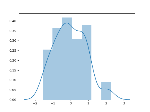
Distribution of Tajima’s D from msprime¶

import msprime
import libsequence
import seaborn as sns

D = []

for ts in msprime.simulate(100, num_replicates=100,
                           mutation_rate=25.0,
                           random_seed=42):
    m = libsequence.VariantMatrix.from_TreeSequence(ts)
    ac = m.count_alleles()
    D.append(libsequence.tajd(ac))

sns.distplot(D)

(Source code)

“Sliding window” analysis¶

To analyze different genomic intervals, or “windows”, you have two options. Any statistic needing the allele count data can easily be gotten via a slice of your existing data:

In [19]: lefts = np.arange(0, 1, 0.2)

In [20]: for l in lefts:
   ....:     p = np.where((vm.positions >= l)&(vm.positions < l+0.2))[0]
   ....:     ac_slice=ac[p[0]:p[-1]+1]
   ....:     assert len(ac_slice) == len(p)
   ....:     print(libsequence.thetapi(ac_slice))
   ....: 
179.54282828282925
198.07858585858628
230.90202020202207
196.7565656565662
175.0989898989905

We may also use libsequence.VariantMatrix.window() to obtain new VariantMatrix instances corresponding to sub-windows of the data:

In [21]: for l in lefts:
   ....:     w = vm.window(l, l+0.2)
   ....:     acw = w.count_alleles()
   ....:     print(libsequence.thetapi(acw))
   ....: 
179.54282828282925
198.07858585858628
230.90202020202207
196.7565656565662
175.0989898989905

Window creation is \(O(log(vm.nsites))\) in time and has trivial additional memory requirements, as the returned object does not own its own data buffer.

Other useful statistics¶

Some more complex descriptors of the data are available

In [22]: diffs = libsequence.difference_matrix(vm)

Here, diffs contains data for representing the distance matrix for the data. Specifically, these values can be used to fill the upper triangle of a matrix:

In [23]: dm = np.array(diffs, dtype=np.int32)

In [24]: m = np.array([0]*(vm.nsam*vm.nsam))

# Get the indices of the upper-diagonal
# of an nsam*nsam matrix, ignoring
# the diagonal:
In [25]: idx = np.triu_indices(vm.nsam,k=1)

In [26]: m=m.reshape((vm.nsam,vm.nsam))

In [27]: m[idx]=dm

In [28]: print(m)
[[   0 1053  940 ...  940  901 1017]
 [   0    0 1037 ... 1023  898 1038]
 [   0    0    0 ... 1102 1031 1101]
 ...
 [   0    0    0 ...    0  853  893]
 [   0    0    0 ...    0    0 1074]
 [   0    0    0 ...    0    0    0]]

# Let's confirm our results via brute-force:
In [29]: gm = ts.genotype_matrix()

In [30]: dummy = 0

In [31]: for i in range(gm.shape[1]-1):
   ....:     for j in range(i+1,gm.shape[1]):
   ....:         diffs = np.where(gm[:,i] != gm[:,j])
   ....:         assert(len(diffs[0])==dm[dummy])
   ....:         dummy+=1
   ....: 

In a similar fashion, we can obtain true/false data on whether pairs of haplotypes differ:

In [32]: diff_yes_or_no = libsequence.is_different_matrix(vm)

libsequence.is_different_matrix(m: libsequence._libsequence.VariantMatrix) → List[int]¶

Return whether or not pairs of samples in a VariantMatrix differ

Parameters:	m – A `libsequence.VariantMatrix`

The contents of this matrix have the exact same layout as diffs described above. The difference is that the data elements are encoded as 0 = identical, 1 = different. This calculation is much faster than the previous.

Note

Missing data do not contribute to samples being considered different, nor to the number of differences.

It is also possible to get a unique label assigned to each haplotype:

In [33]: labels = np.array(libsequence.label_haplotypes(vm),dtype=np.int32)

In [34]: print(len(np.unique(labels)))
99

libsequence.label_haplotypes(arg0: libsequence._libsequence.VariantMatrix) → List[int]¶

Internally, the results from is_different_matrix are used to assign the labels.

These labels are likewise used internally to count the number of haplotypes:

In [35]: print(libsequence.number_of_haplotypes(vm))
99

# Confirm result via direct comparison to
# the data from msprime:
In [36]: print(len(np.unique(gm.transpose(),axis=0)))
99

What about performance?

In [37]: %timeit -n 10 -r 10 libsequence.number_of_haplotypes(vm)
10 loops, best of 10: 271 us per loop

In [38]: %timeit -n 10 -r 10 len(np.unique(gm.transpose(),axis=0))
10 loops, best of 10: 11.3 ms per loop

Calculating summary statistics¶

Simple overview of concepts¶

List of “classic”/standard summary statistics¶

Distribution of Tajima’s D from msprime¶

“Sliding window” analysis¶

Other useful statistics¶

Table of Contents

Previous topic

Next topic

This Page