3. Pedigrees and “gene trees”

Fig. 3.1 shows a simple pedigree called a “trio.” Trios consist of two parents with a single offspring. This pedigree uses standard notation:

1. Males (individuals producing sperm) are shown as squares.

2. Females (individuals producing eggs) are shown as circles.

The individuals in the pedigree have numeric labels starting with 1 (one). Individuals at the top of the pedigree are ancestors to those appearing nearer the bottom.

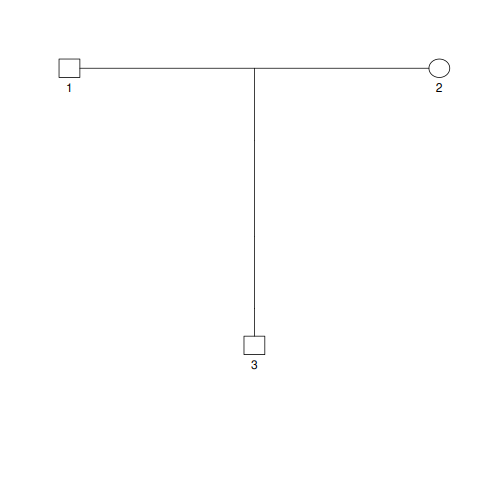
Fig. 3.1 A “trio” pedigree.

The edges that connect parents to children in a pedigree represent meiosis. In other words, parental chromosomes were replicated (and mutated and recombined), and then a single new chromosome was passed down to an offspring.

If we consider the case of autosomal inheritance in diploid organisms like humans, then each individual contains two copies of the genome, one inherited via sperm and the other via egg.

The principles of Mendelian inheritance tell us that:

1. The two parents in Fig. 3.1 each have two genomes. Let’s label the genomes of parent 1 as 1 and 2. Let’s label the genomes of parent 2 as 3 and 4.

2. Ignoring some details of meiosis for now (mutation and recombination), individual 3 will inherit genome 1 half the time and genome 2 half the time from parent 1. Likewise, parent 1 will pass on either genome 3 or genome 4 with equal probability.

When discussing autosomal inheritance in diploids, we will adopt the following convention for genome labels:

• For an individual in the pedigree with label \(i\), that individual’s two genomes will be labelled \(2i - 1\) and \(2i\)

For example, individual 7 in a pedigree will have genomes \(2\times 7 - 1 = 13\) and \(2\times 7 = 14\). This convention will allow us to track both genes and individuals.

Fig. 3.2 An example of genome inheritance, given the pedigree structure in Fig. 3.1. The node labels are individual: genome. The values given for genome follow the convention described in the main text and individual labels are identical to Fig. 3.1.

Figure Fig. 3.2 shows an example of “gene dropping” applied to the pedigree from Fig. 3.1. Following our labelling convention described above, we see that the offspring individual (number 3) inherited its first genome (3) from genome 2 which was found in the parent individual labelled 1. The other genome came from genome 3 in individual 2.

Figure Fig. 3.2 is a new type of graph that we may call a “gene tree”. The nodes in a gene tree usually refer to gene (or genome) sequences and their ancestors. Figure Fig. 3.2 takes the extra step of tracking the specific individual to which each genome belongs or belonged.

Fundamentally, gene trees display:

1. Nodes, which refer to genomes.

2. The height of the node in the tree indicate its birth time. In Fig. 3.2, the y axis is in units of generations in the past. Thus, the genomes belonging to the parents exist (or existed) one generation ago. Each node gets a unique label.

3. Edges display the transmission of one genome to another.

Attention

Caution!

It is important to remember the following points when thinking about gene trees and their associated pedigrees:

• A given pedigree has a fixed structure that describes the familial relationships.

• This pedigree structure constrains the pathways for gene inheritance. (Genes are only inherited from parents.)

• The gene trees for a given pedigree shown in this document are examples. There are many possible gene trees for a given pedigree. For a single nonrecombining segment of DNA, there is only a 50% chance that it is passed to an offspring. When a family has more than one offspring, a given DNA segment may be passed to 0, 1, 2, etc., offspring.

• We often only have DNA data from the most recent generation of a pedigree. We therefore have to consider multiple possible pathways by which that information passed from the founders to our genotyped individuals.

Fig. 3.3 shows a pedigree with two siblings. Fig. 3.4 and Fig. 3.5 show two examples of genome inheritance given this pedigree. In Fig. 3.4 , both offspring inherit the same two alleles while in Fig. 3.5, the two siblings inherit different alleles from each parent for both of their genomes.

Attention

Take a moment to practice! It is probably a good idea to make sure that you really understand what these images are showing. Instead of skimming over the graphics, take some time to make sure that you understand how the individual: genome annotations in Fig. 3.4 and Fig. 3.5 map on to the pedigree in Fig. 3.3.

See Section 9 if you need more help on how these images work.

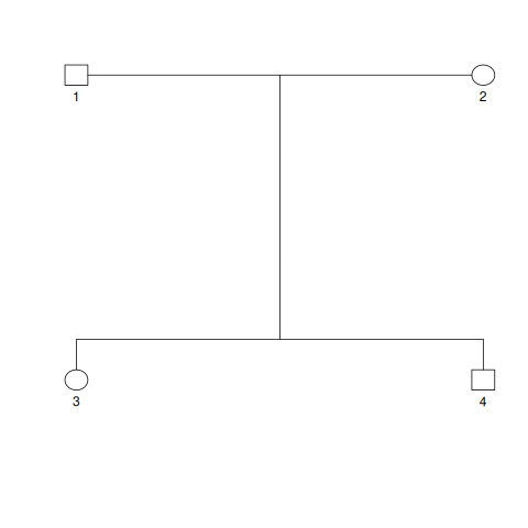
Fig. 3.3 A pedigree with two siblings.

Fig. 3.4 One example of “gene dropping” onto the pedigree from Fig. 3.3.

Fig. 3.5 Another example of “gene dropping” onto the pedigree from Fig. 3.3.

The pedigree shown in Fig. 3.6 shows multiple generations of a family, ending with two sets of cousins. Individuals 11 and 12 are first cousins (sharing grandparents) to individuals 13 and 14.

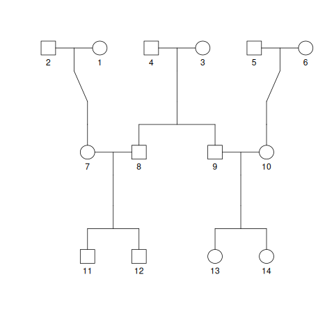
Fig. 3.6 A multigeneration pedigree.

Starting with these sets of cousins, we can imagine starting to trace their genomes back in time until we reach the grand-parental generation. For example, for each genome of the two genomes in individual 11, the genome came either from individual 7 or from 8. If it came from 7, then we know that it came from one of the two grandparents labelled 1 or 2. But if it came from 8, then the grandparent of that genome was either 3 or 4. Therefore, in order for our cousins to have inherited a genome from the same common ancestor, the pathways of inheritance for those genomes must trace back to the grandparent couple 3 and 4. Further, the genomes must come from the same grandparent and then they must come from the same genome from that shared grandparent. If all of this happens, then we say that the two genomes have “coalesced” into their common ancestor.

Fig. 3.7 shows the result of “gene dropping” onto this pedigree. We see that all four cousins share a genome descended from genome 5 of grandparent 3.

The tree in Fig. 3.7 shows several interesting features:

• Our pedigree (Fig. 3.6) contains six grandparents (two generations ago), yet only four of them (individuals 2, 3, 5, and 6) contributed alleles to the grandchildren.

• For those grandparents that did contribute to the genomes of their grandchildren, all of them only passed on one of their two possible alleles.

• Turning to the parental generation (1 generation ago), we see that all four parents contributed genes to the final generation, yet only individual 10 passed on a copy of each of their alleles.

• There are multiple occasions where a single allele was passed on to more than one offspring. For example, allele 5 was passed from individual 3 to individuals 8 and 9. When an allele is transmitted to multiple descendant nodes, we get a branching pattern in our tree. When an allele is transmitted to only a single descendant in the tree, we get straight lines, or “unary transmission” of the gene copy. An example of unary transmission starts with allele 11 in grandparent 6. It is passed to individual 10, becoming allele 20. It is then passed on to individual 14, becoming allele 28.

• There are 4 distinct trees shown in this image!

Fig. 3.7 Genome inheritance on the pedigree from Fig. 3.6.

We may also note that much of the information in Fig. 3.7 is not especially useful in understanding the ancestry of the alleles found in our present-day individuals (those born 0 generations ago). There are many unary nodes, including unary nodes ancestral to nodes associated with branching events. Fig. 3.8 shows a “simplified” version of this image with unary transmission events removed and we stop at the most recent common ancestor of any set of nodes. This simplified tree is the minimal graph that we require to describe the ancestral history of the alleles in our present-day individuals. This simplified representation illustrates an important concept – the important information in a gene tree is the branching structure that illustrates the relationship among our sample of alleles/genomes. This branching relationship is completely analogous to what we discussed for species trees in Section 2.

Fig. 3.8 The tree(s) from Fig. 3.7 simplified to only show non-unary inheritance and to stop at the most recent common ancestor of each node.

Fig. 3.7 and Fig. 3.8 also reveal something that may be surprising. These gene trees come from a small familial pedigree (Fig. 3.6). However, we noted above that only 3/4 of the grandparents have directly contributed DNA to the most recent generation. In other words, “direct” DNA connections to even recent ancestors are quickly lost. This loss is due to the randomness of the “Mendelian lottery”. At an autosomal locus a given allele is only passed on to half of an individual’s offspring. Further, humans tend to have few offspring. Few offspring implies few chances to pass on genes, meaning that there is a high likelihood that an individual does not pass both of their alleles on to the next generation.