4. Pedigrees in randomly mating populations#
The pedigrees and gene trees discussed in Section 3 were the standard familial pedigrees that we are used to from medical genetics.
In this section, we look at pedigrees that are the random outcome of an evolutionary model. We get the pedigrees by computer simulation.
In words the details of the model are:
There are \(N\) diploid founder individuals.
For all but the final generation, exactly \(N/2\) individuals are female and the remaining \(N/2\) are male.
\(N\) does not change each generation.
To generate the next generation:
Randomly pair each female with exactly one male, forming monogamous pairings.
Each pair has the same average fecundity (number of offspring).
We keep sampling pairs at random and recording births until we have made \(N\) offspring.
We track the parents of each offspring each generation
For the final generation, we randomly assign male/female status.
Using the simulated outputs, we can make the same kinds of plots that we discussed in Section 3
4.1. A small example#
Fig. 4.1 shows a pedigree with 4 founders and a total of 4 generations. You will notice some individuals connected by two horizontal lines instead of the usual one. Due to the small population size (\(N\)), close relatives may be paired as parents. We say that offspring of such pairings are the product of “consanguineous” matings, which is just another way of saying inbreeding. The two horizontal lines indicate parings that result in inbred offspring.
Fig. 4.2 and Fig. 4.3 show the unsimplified and simplified patterns of allele transmission, respectively. These graphics should look very similar to those from Section 3, showing rapid loss of both genealogical and genetic ancestors.
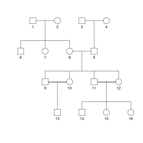
Fig. 4.1 A random pedigree starting with 4 founders and then evolving for 3 more generations of random mating. The double horizontal lines indicate parents that are close relatives. Their offspring are therefore inbred.#

Fig. 4.2 An unsimplified gene tree from the pedigree in Fig. 4.1.#

Fig. 4.3 The simplified version of the gene trees from Fig. 4.2.#
4.2. A larger example#
Fig. 4.4 shows a pedigree with 6 founders and 10 generations of random mating. The gene trees are in Fig. 4.5 and Fig. 4.6.

Fig. 4.4 A random pedigree starting with 6 founders and then evolving for 9 more generations of random mating. The double horizontal lines indicate parents that are close relatives. The arcs connect an individual from where it occurs in a sibship (the set of offspring of a given pair of parents) to where that same individual is a parent. The arcs are necessary due to the density of individuals in the pedigree.#

Fig. 4.5 An unsimplified gene tree from the pedigree in Fig. 4.4.#
As with the smaller example in the previous section, we see rapid loss of ancestry. However, we should note that, of the 10 generations of random mating, we the common ancestors of individual alleles are obtained by at most 4 generations into the past (Fig. 4.6).

Fig. 4.6 The simplified version of the gene trees from Fig. 4.5.#
4.3. Pedigrees and population genetics#
The previous sections on pedigrees and gene trees illustrate that there are two genealogical structures in natural populations. First, there is the pedigree, which is a graph representing the relationships among individuals. Second, there is a “gene tree” of the actual transmission of DNA across generations.
The field of population genetics is mostly concerned with the second structure (the gene tree). While it is recognized that the structure of this gene tree depends on the structure of the true pedigree of the population, we rarely have detailed information about pedigrees. What we can obtain rather easily is genetic information from contemporary individuals. In some cases, we can also obtain genetic information from ancient individuals. For example, it is relatively common now to sequence “ancient DNA” from human remains. In some cases, the samples are over 1000 years old! We also now have draft genome sequences of individuals from extinct hominid species such as the Neanderthal. Much of modern population genetics involves making inferences about the evolutionary history of one or more populations using such genomic data.