6. Population graphs#
When thinking about the evolution of a species, we need a way to conceptualize the relationships among different populations across the species’ geographic range. Our empirical studies usually involve contemporary samples (individuals) from one or more locations of this range. We often describe our samples using rather simplistic language. For example, “20 Drosophila melanogaster from Raleigh, North Carolina and 15 from Zimbabwe, Africa”. An example of human population labels is shown in Table 6.1.
Label |
Description |
|---|---|
AMH |
Anatomically modern humans |
OOA |
Out of Africa population |
YRI |
Yoruba in Ibadan, Nigera |
CEU |
Utah Residents (CEPH) with Northern and Western European ancestry |
CHB |
Han Chinese in Beijing, China |
Given a set of such population labels, we will attempt to describe the historical relationship between the locations that our samples come from. To do this, we will often envision a picture that contains information such as when our populations diverged from some common ancestral population, the history of changing population size in each population, and the history of migration events over time. Ignoring many important technical details, once we write down such a model, we can infer the parameters of the model using genotype data from our sampled individuals. Briefly, features of the data such as the similarities and differences in the frequencies of mutations are impacted by the demographic history. Therefore, we can “work backwards” to infer the details of a specific model given such data.
Fig. 6.1 shows a demographic history inferred from genotype data from three contemporary populations by Jouganous et al. [JLRG17].
The population labels are in Table 6.1.
The contemporary populations are YRI, CHB, and CEU.
The OOA and AMH populations are part of the model and not a population from which we have samples.
We know from many lines of evidence a subset of our ancestors left Africa, settled in what is now called the Middle East, and from there spread to the rest of the world.
Our model makes a set of simplifying assumptions:
Contemporary Yoruba are the direct descendants of “anatomically modern humans”, or
AMH, which is modeled as a single ancestral source of our species.At some point in the past, some individuals “branched off” from
AMH, leaving Africa. ThisOOApopulation may been small.The contemporary non-African populations then branched off from
OOAto populate Europe and Asia. The spreading through these continents is modeled as exponential population growth.Migration is allowed between populations when they coexist.
Fig. 6.1 is the result of using the genotype data to inform use about specific values for each of these parameters.
Pictures like Fig. 6.1 are graphs that describe a demographic history. When the parameters of the graph are inferred from data, it is important that we recognize the following:
The graph cannot be said to be the “true history” of humans! The models make several simplifying assumptions. For example, they ignore that populations of individuals exist in continuous space and instead assume that individuals can be treated as existing within discrete populations that interact in simple ways.
Further, the parameters belong to a certain “picture” (model). Adding more features to, or taking features away from, the model will change the parameter estimates. Adding and subtracting model features creates a new model. We currently do not have effective methods for evaluating large numbers of models to find the “best” one. We know from computer simulations that we can accurately infer the parameters of models like Fig. 6.1 if such a model is the truth. But model selection, or choosing the best model from a large set, is very difficult. The difficulty exists in part because the search space of models is infinitely large!
The above list may these parameter inferences not sound very useful. However:
If we simulate data from the model plus its inferred parameters, we get out data that matches many important features of our input data.
In many cases, such simulations also predict features of our data that were not used for inference.
In other words, the parameters inferred using these simplified models have some predictive ability, and that is very useful. As we gather more data from contemporary populations, we can ask if our old models predict features of our new data. If we obtain data from ancient samples (human remains preserved in a bog in Northern Europe, for example), we can also ask if those genotypes are consistent with what we’d expect from samples of that age. If not, we can refine our models.
The previous paragraphs focus the discussion on inferences about the detailed history of populations. Interest in studying population history for the sole sake of understanding that history is largely limited to humans. In other study systems, we typically only concern ourselves with such inferences if they have scientific or policy implications. For example, it may be useful to know something about the history of endangered bird or insect species in order to make decisions about conservation practices. Scientifically, the interest in demographic inference exists because we are interested in how natural selection affects genome evolution and both demography and selection affect genotype frequencies across populations of the species that we study.
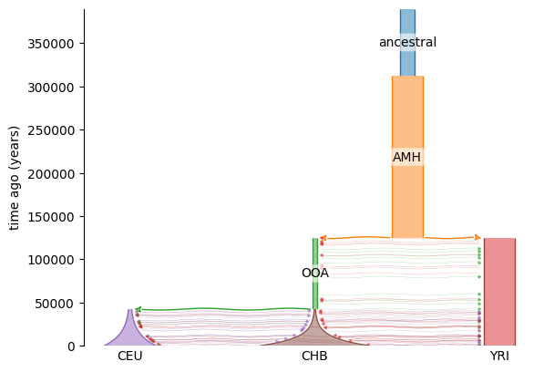
Fig. 6.1 A graphical model of relationships between multiple human populations.
From bottom to top, time moves to the past.
Each population gets a different color and the width is proportional to the population size at a given time in the past.
Thick arrows represent founding events.
For example, the thick green arrow from OOA to CEU means that the latter population arose from the former.
The thinner arrows refer to continuous migration between populations.
The color of the arrow tip refers to the source of migration and the arrow points at the destination.
The population labels are defined in Table 6.1.
The time units are in years assuming a generation time of 29 years per generation.#