The multivariate Gaussian distribution

Show code cell source Hide code cell source

import demes
import demesdraw
import fwdpy11
import numpy as np

We may model Gaussian effect sizes using the existing fwdpy11.MultivariateGaussianEffects in conjunction with fwdpy11.mvDES.

At this time, it is probably best to look at an example. The following code models Gaussian stabilizing selection on a quantitative trait. The effects sizes within each deme are themselves given by Gaussian distributions and there is no correlation in the effect size in the two demes.

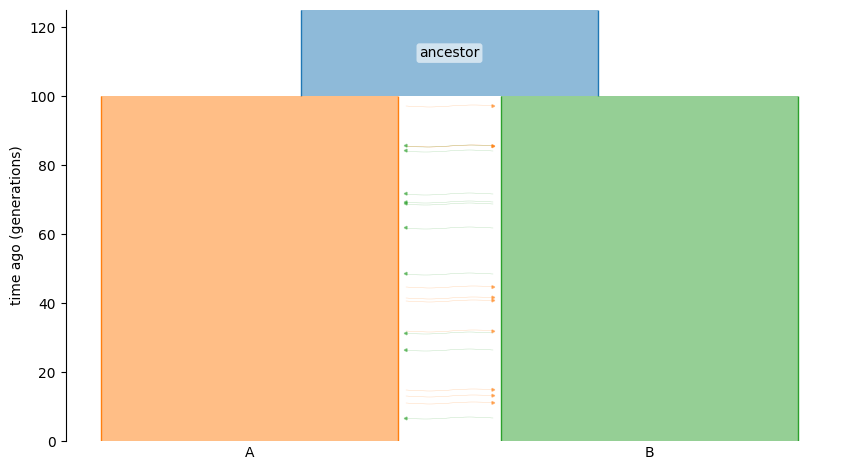
We will simulate a demographic model of migration happening into the infinite past of two equal-sized demes:

Show code cell source Hide code cell source

yaml = """
description: Island model forever
time_units: generations
demes:
  - name: ancestor
    epochs:
     - start_size: 100
       end_time: 100
  - name: A
    ancestors: [ancestor]
    epochs:
     - start_size: 100
  - name: B
    ancestors: [ancestor]
    epochs:
     - start_size: 100
migrations:
  - demes: [A, B]
    rate: 0.10
"""
g = demes.loads(yaml)
model = fwdpy11.ForwardDemesGraph.from_demes(g, burnin=1)
demesdraw.tubes(g);

Let’s set up a dictionary to hold the parameters of our model:

pdict = {
    "nregions": [],
    "recregions": [],
    "sregions": [
        fwdpy11.mvDES(
            fwdpy11.MultivariateGaussianEffects(0, 1, 1, np.identity(3)), np.zeros(3)
        )
    ],
    "rates": (0, 2.5e-3, None),
    "demography": model,
    "simlen": model.final_generation,
    "gvalue": fwdpy11.Additive(
        ndemes=3, scaling=2,
        gvalue_to_fitness=fwdpy11.GaussianStabilizingSelection.single_trait([fwdpy11.Optimum(optimum=0.0, VS=10.0, when=0)])
    ),
    "prune_selected": False,
}

Most of the above is standard. Let’s dissect the new bits:

• An instance of fwdpy11.mvDES is our only region with selected mutations.

• This instance holds an instance of fwdpy11.MultivariateGaussianEffects that puts mutations on the interval \([0, 1)\) with weight 1 and an identity matrix specifies the correlation in effect sizes between demes 0 and 1. The identity matrix has the value zero for all off-diagonal elements, meaning no covariance in effect sizes across demes.

• The final constructor argument specifies the mean of each marginal Gaussian distribution. The means are both zero.

• Our genetic value type accepts an ndemes parameter, telling it that it has to look for deme-specific effect sizes. This value must be set to the maximum number of demes that will exist during a simulation.

Let’s evolve the model now:

params = fwdpy11.ModelParams(**pdict)
# TODO: update this once we have a function to pull the sizes
# automatically from demes-derived models:
initial_sizes = model.initial_sizes
pop = fwdpy11.DiploidPopulation(initial_sizes, 1.0)
rng = fwdpy11.GSLrng(1010)
fwdpy11.evolvets(rng, pop, params, 10)

Let’s extract the effect sizes from each deme:

assert len(pop.tables.mutations) > 0
for i in pop.tables.mutations:
    print(pop.mutations[i.key].esizes)

[ 1.33393583 -1.42671084  2.37936694]
[ 0.74651187  0.20938071 -0.7841031 ]
[ 0.32575285  0.35069963 -0.11465527]
[-0.24181509  1.00965354  0.68807326]
[ 1.17357808  0.63700908 -2.40771662]
[-0.22207726  0.23289436  0.92726017]
[ 0.24505205  0.73996041 -0.70205993]
[ 0.5018422   0.50924973 -0.10140017]
[-0.22408902  0.83343064 -0.2691579 ]

Let’s look at another example where effect sizes covary negatively across demes and raise the mutation rate a bit:

# Effect sizes across demes will
# have a correlation coefficient of r=1/2
cor_matrix = np.array([-0.5]*9).reshape(3,3)
np.fill_diagonal(cor_matrix, np.array([1.0]*3))

# Get our covariance matrix
sd = np.array([0.1]*3)
D = np.identity(3)
np.fill_diagonal(D, sd)
vcv_matrix = np.matmul(np.matmul(D, cor_matrix), D)
pdict["sregions"] = [
    fwdpy11.mvDES(fwdpy11.MultivariateGaussianEffects(0, 1, 1, vcv_matrix), np.zeros(3))
]
params = fwdpy11.ModelParams(**pdict)
# TODO: update this once we have a function to pull the sizes
# automatically from demes-derived models:
initial_sizes = model.initial_sizes
pop = fwdpy11.DiploidPopulation(initial_sizes, 1.0)
fwdpy11.evolvets(rng, pop, params, 10)
for i in pop.tables.mutations:
    print(pop.mutations[i.key].esizes)

[-0.07440418  0.03966954  0.03473464]
[ 0.07414971  0.06569778 -0.13984749]
[ 0.07593905 -0.04116704 -0.03477201]
[ 0.13958957 -0.22582578  0.08623621]
[-0.02982778  0.0895709  -0.05974312]
[-0.08529108  0.14513978 -0.05984871]
[ 0.06425309  0.01562452 -0.07987761]
[ 0.01898601  0.07154382 -0.09052983]

Now we see that the effect sizes often differ in sign between the two demes.