Mutations with variable dominance

New in version 0.13.0.

The heterozygous effect of a mutation does not need to be constant. You may use instances of classes derived from fwdpy11.MutationDominance to assign functions to generate the dominance of mutations.

The available classes are:

• fwdpy11.FixedDominance This class is equivalent to passing in a float to the h kwarg. See here

• fwdpy11.ExponentialDominance

• fwdpy11.UniformDominance

• fwdpy11.LargeEffectExponentiallyRecessive

Example

import fwdpy11

des = fwdpy11.GaussianS(beg=0, end=1, weight=1, sd=0.1,
    h=fwdpy11.LargeEffectExponentiallyRecessive(k=5.0))

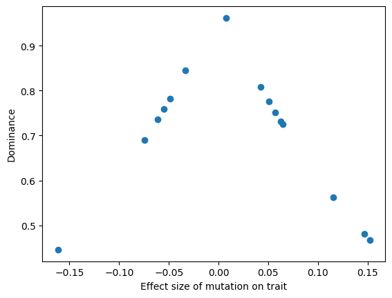
If we apply this des object to a model of a quantitative trait evolving to a sudden “optimum shift”, then we see that the larger effect variants present at the end of the simulation to indeed have smaller dominance coefficients.

Show code cell source Hide code cell source

pop = fwdpy11.DiploidPopulation(500, 1.0)

rng = fwdpy11.GSLrng(54321)

GSSmo = fwdpy11.GSSmo(
    [
        fwdpy11.Optimum(when=0, optimum=0.0, VS=1.0),
        fwdpy11.Optimum(when=10 * pop.N - 200, optimum=1.0, VS=1.0),
    ]
)

rho = 1000.

p = {
    "nregions": [],
    "gvalue": fwdpy11.Additive(2.0, GSSmo),
    "sregions": [des],
    "recregions": [fwdpy11.PoissonInterval(0, 1., rho / float(4 * pop.N))],
    "rates": (0.0, 1e-3, None),
    "prune_selected": False,
    "demography": fwdpy11.ForwardDemesGraph.tubes([pop.N], burnin=10),
    "simlen": 10 * pop.N,
}
params = fwdpy11.ModelParams(**p)

fwdpy11.evolvets(rng, pop, params, 100, suppress_table_indexing=True)

Show code cell source Hide code cell source

import matplotlib.pyplot as plt
esize = [pop.mutations[m.key].s for m in pop.tables.mutations]
h = [pop.mutations[m.key].h for m in pop.tables.mutations]

f, ax = plt.subplots()
ax.scatter(esize, h)
ax.set_xlabel("Effect size of mutation on trait")
ax.set_ylabel("Dominance")
plt.show();

Using discrete distributions

fwdpy11.DiscreteDESD specifies a Discrete Effect Size and Dominance joint distribution. A list of tuple of (effect size, dominance, weight) specify the joint distribution. For example:

import math
import numpy as np

joint_dist = []
for s in np.arange(0.1, 1, 0.1):
    joint_dist.append((-s, math.exp(-s), 1./s))

des = fwdpy11.DiscreteDESD(beg=0, end=1, weight=1, joint_dist=joint_dist)
print(des.asblack())

fwdpy11.DiscreteDESD(
    beg=0,
    end=1,
    weight=1,
    joint_dist=[
        (-0.1, 0.9048374180359595, 10.0),
        (-0.2, 0.8187307530779818, 5.0),
        (-0.30000000000000004, 0.7408182206817179, 3.333333333333333),
        (-0.4, 0.6703200460356393, 2.5),
        (-0.5, 0.6065306597126334, 2.0),
        (-0.6, 0.5488116360940264, 1.6666666666666667),
        (-0.7000000000000001, 0.49658530379140947, 1.4285714285714284),
        (-0.8, 0.44932896411722156, 1.25),
        (-0.9, 0.4065696597405991, 1.1111111111111112),
    ],
    coupled=True,
    label=0,
    scaling=1.0,
)

The result is that mutations with smaller effect sizes are more common (larger weights) and more dominant.