Recording data during a simulation

In order to facilitate time-series analyses, you may pass a callable object to fwdpy11.evolvets(). The following boiler plate illustrates the requirements for the callable objects in both Python and in C++:

python

class Recorder(object):
    def __call__(self, pop: fwdpy11.DiploidPopulation, sampler: fwdpy11.SampleRecorder):
        pass

c++

#include <fwdpy11/evolvets/SampleRecorder.hpp>
#include <fwdpy11/types/DiploidPopulation.hpp>

struct Recorder {
    void operator()(const fwdpy11::DiploidPopulation & pop,
                    fwdpy11::SampleRecorder & sampler)
    {
    }
};

The remainder of this vignette will only cover Python. The arguments to __call__ are an instance of fwdpy11.DiploidPopulation and fwdpy11.SampleRecorder, respectively. The latter allows one to record “ancient samples” during a simulation, which we discuss more below.

Note

Given that you can pass in any valid Python object, you can record anything you can imagine based on attributes of fwdpy11.DiploidPopulation. Further, as many of those attributes can be viewed as numpy.ndarray or numpy.recarray, you may use any Python library compatible with those types.

You can also process the genealogy of the population. Doing so is an advanced topic, which we deal with in a later vignette.

Todo

Write vignette showing how to access the tree sequences during a simulation.

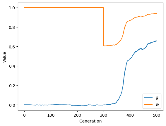
Let’s return to the model from the previous vignette. We will implement a recorder to track the mean trait value and fitness of the entire population over time.

That recorder object will look like this:

import fwdpy11
import numpy as np

class Recorder(object):
    def __init__(self):
        self.generation = []
        self.mean_trait_value = []
        self.mean_fitness = []
        
    def __call__(self, pop, sampler):
        md = np.array(pop.diploid_metadata, copy=False)
        self.generation.append(pop.generation)
        self.mean_trait_value.append(md['g'].mean())
        self.mean_fitness.append(md['w'].mean())

The details of the simulation model follow, but are hidden by default as they repeat material from the previous vignette.

Show code cell source Hide code cell source

pop = fwdpy11.DiploidPopulation(500, 1.0)

rng = fwdpy11.GSLrng(54321)

GSSmo = fwdpy11.GSSmo(
    [
        fwdpy11.Optimum(when=0, optimum=0.0, VS=1.0),
        fwdpy11.Optimum(when=pop.N - 200, optimum=1.0, VS=1.0),
    ]
)

rho = 1000.

des = fwdpy11.GaussianS(beg=0, end=1, weight=1, sd=0.1,
    h=fwdpy11.LargeEffectExponentiallyRecessive(k=5.0))

p = {
    "nregions": [],
    "gvalue": fwdpy11.Additive(2.0, GSSmo),
    "sregions": [des],
    "recregions": [fwdpy11.PoissonInterval(0, 1., rho / float(4 * pop.N))],
    "rates": (0.0, 1e-3, None),
    "prune_selected": False,
    "demography": fwdpy11.ForwardDemesGraph.tubes([pop.N], burnin=1),
    "simlen": pop.N,
}
params = fwdpy11.ModelParams(**p)

We now pass in our callable to fwdpy11.evolvets():

recorder = Recorder()
fwdpy11.evolvets(rng, pop, params, recorder=recorder, simplification_interval=100) 

Plotting our results:

import matplotlib.pyplot as plt

f, ax = plt.subplots()
ax.plot(recorder.generation, recorder.mean_trait_value, label=r'$\bar{g}$')
ax.plot(recorder.generation, recorder.mean_fitness, label=r'$\bar{w}$')
ax.set_xlabel('Generation')
ax.set_ylabel('Value')
ax.legend(loc='best');

Recording ancient samples

Let’s write a new class that “preserves” a random number of individuals each generation. This recording preserves their nodes in the fwdpy11.TableCollection and their meta data in fwdpy11.DiploidPopulation.ancient_sample_metadata.

Our class will also do all of the same operations that Recorder did.

class RandomSamples(object):
    def __init__(self, nsam):
        self.nsam = nsam
        self.generation = []
        self.mean_trait_value = []
        self.mean_fitness = []
        
    def __call__(self, pop, sampler):
        md = np.array(pop.diploid_metadata, copy=False)
        self.generation.append(pop.generation)
        self.mean_trait_value.append(md['g'].mean())
        self.mean_fitness.append(md['w'].mean())
        sampler.assign(np.random.choice(pop.N, self.nsam, replace=False))

To run this, we first create a new population, random number generator, and model parameters object. We need a new model parameters instance because the one used above has already applied the optimum shift. Thus, we need to rebuild the gvalue field.

import pickle
pop = fwdpy11.DiploidPopulation(500, 1.0)
rng = fwdpy11.GSLrng(54321)
p['gvalue'] = fwdpy11.Additive(2.0, GSSmo)
params = fwdpy11.ModelParams(**p)
recorder = RandomSamples(5)
fwdpy11.evolvets(rng, pop, params, recorder=recorder, simplification_interval=100) 

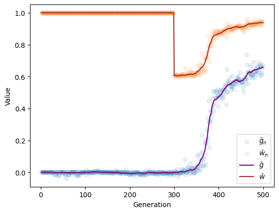
We now want to recreate the plot from above, but with the values from our ancient samples shown as dots. Analyzing each time point separately is a common operation made easier by fwdpy11.DiploidPopulation.sample_timepoints().

ancient_generation = []
ancient_mean_trait_value = []
ancient_mean_fitness = []
for g, nodes, md in pop.sample_timepoints(include_alive=False):
    ancient_generation.append(g)
    ancient_mean_trait_value.append(md['g'].mean())
    ancient_mean_fitness.append(md['w'].mean())

Finally, the plot:

f, ax = plt.subplots()
ax.scatter(ancient_generation, ancient_mean_trait_value,
           alpha=0.1, label=r'$\bar{g}_{n}$')
ax.scatter(ancient_generation, ancient_mean_fitness,
           alpha=0.1, label=r'$\bar{w}_{n}$')
ax.plot(recorder.generation, recorder.mean_trait_value,
        color='purple',
        alpha=1, label=r'$\bar{g}$')
ax.plot(recorder.generation, recorder.mean_fitness,
        color='brown',
        alpha=1, label=r'$\bar{w}$')
ax.set_xlabel('Generation')
ax.set_ylabel('Value')
ax.legend(loc='best');

Built-in ancient sample recorders

• fwdpy11.RandomAncientSamples